Chapter 3 Tables, Graphics, References, and Labels
3.1 Tables
In addition to the tables that can be automatically generated from a data frame in R that you saw in R Markdown Basics using the kable() function, you can also create tables using pandoc. (More information is available at https://pandoc.org/README.html#tables.) This might be useful if you don’t have values specifically stored in R, but you’d like to display them in table form. Below is an example. Pay careful attention to the alignment in the table and hyphens to create the rows and columns.
| Factors | Correlation between Parents & Child | Inherited |
|---|---|---|
| Education | -0.49 | Yes |
| Socio-Economic Status | 0.28 | Slight |
| Income | 0.08 | No |
| Family Size | 0.18 | Slight |
| Occupational Prestige | 0.21 | Slight |
We can also create a link to the table by doing the following: Table 3.1. If you go back to Loading and exploring data and look at the kable table, we can create a reference to this max delays table too: Table 1.1. The addition of the (\#tab:inher) option to the end of the table caption allows us to then make a reference to Table \@ref(tab:label). Note that this reference could appear anywhere throughout the document after the table has appeared.
3.2 Figures
If your thesis has a lot of figures, R Markdown might behave better for you than that other word processor. One perk is that it will automatically number the figures accordingly in each chapter. You’ll also be able to create a label for each figure, add a caption, and then reference the figure in a way similar to what we saw with tables earlier. If you label your figures, you can move the figures around and R Markdown will automatically adjust the numbering for you. No need for you to remember! So that you don’t have to get too far into LaTeX to do this, a couple R functions have been created for you to assist. You’ll see their use below.
In the R chunk below, we will load in a picture stored as reed.jpg in our main directory. We then give it the caption of “Reed logo”, the label of “reedlogo”, and specify that this is a figure. Make note of the different R chunk options that are given in the R Markdown file (not shown in the knitted document).

Figure 3.1: Reed logo
Here is a reference to the Reed logo: Figure 3.1. Note the use of the fig: code here. By naming the R chunk that contains the figure, we can then reference that figure later as done in the first sentence here. We can also specify the caption for the figure via the R chunk option fig.cap.
Below we will investigate how to save the output of an R plot and label it in a way similar to that done above. Recall the flights dataset from Chapter 1. (Note that we’ve shown a different way to reference a section or chapter here.) We will next explore a bar graph with the mean flight departure delays by airline from Portland for 2014.
mean_delay_by_carrier <- flights %>%
  group_by(carrier) %>%
  summarize(mean_dep_delay = mean(dep_delay))
ggplot(mean_delay_by_carrier, aes(x = carrier, y = mean_dep_delay)) +
  geom_bar(position = "identity", stat = "identity", fill = "red")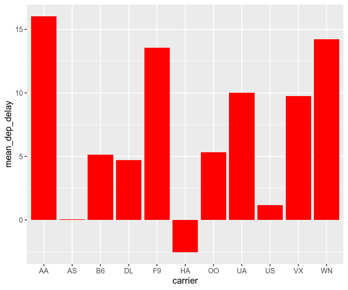
Figure 3.2: Mean Delays by Airline
Here is a reference to this image: Figure 3.2.
A table linking these carrier codes to airline names is available at https://github.com/ismayc/pnwflights14/blob/master/data/airlines.csv.
Next, we will explore the use of the out.extra chunk option, which can be used to shrink or expand an image loaded from a file by specifying "scale= ". Here we use the mathematical graph stored in the “subdivision.pdf” file.
Figure 3.3: Subdiv. graph
Here is a reference to this image: Figure 3.3. Note that echo=FALSE is specified so that the R code is hidden in the document.
More Figure Stuff
Lastly, we will explore how to rotate and enlarge figures using the out.extra chunk option. (Currently this only works in the PDF version of the book.)
Figure 3.4: A Larger Figure, Flipped Upside Down
As another example, here is a reference: Figure 3.4.
3.3 Footnotes and Endnotes
You might want to footnote something.1 The footnote will be in a smaller font and placed appropriately. Endnotes work in much the same way. More information can be found about both on the CUS site or feel free to reach out to data@reed.edu.
3.4 Bibliographies
Of course you will need to cite things, and you will probably accumulate an armful of sources. There are a variety of tools available for creating a bibliography database (stored with the .bib extension). In addition to BibTeX suggested below, you may want to consider using the free and easy-to-use tool called Zotero. The Reed librarians have created Zotero documentation at https://libguides.reed.edu/citation/zotero. In addition, a tutorial is available from Middlebury College at https://sites.middlebury.edu/zoteromiddlebury/.
R Markdown uses pandoc (https://pandoc.org/) to build its bibliographies. One nice caveat of this is that you won’t have to do a second compile to load in references as standard LaTeX requires. To cite references in your thesis (after creating your bibliography database), place the reference name inside square brackets and precede it by the “at” symbol. For example, here’s a reference to a book about worrying: (Molina & Borkovec, 1994). This Molina1994 entry appears in a file called thesis.bib in the bib folder. This bibliography database file was created by a program called BibTeX. You can call this file something else if you like (look at the YAML header in the main .Rmd file) and, by default, is to placed in the bib folder.
For more information about BibTeX and bibliographies, see our CUS site (https://web.reed.edu/cis/help/latex/index.html)2. There are three pages on this topic: bibtex (which talks about using BibTeX, at https://web.reed.edu/cis/help/latex/bibtex.html), bibtexstyles (about how to find and use the bibliography style that best suits your needs, at https://web.reed.edu/cis/help/latex/bibtexstyles.html) and bibman (which covers how to make and maintain a bibliography by hand, without BibTeX, at https://web.reed.edu/cis/help/latex/bibman.html). The last page will not be useful unless you have only a few sources.
If you look at the YAML header at the top of the main .Rmd file you can see that we can specify the style of the bibliography by referencing the appropriate csl file. You can download a variety of different style files at https://www.zotero.org/styles. Make sure to download the file into the csl folder.
Tips for Bibliographies
- Like with thesis formatting, the sooner you start compiling your bibliography for something as large as thesis, the better. Typing in source after source is mind-numbing enough; do you really want to do it for hours on end in late April? Think of it as procrastination.
- The cite key (a citation’s label) needs to be unique from the other entries.
- When you have more than one author or editor, you need to separate each author’s name by the word “and” e.g.
Author = {Noble, Sam and Youngberg, Jessica},. - Bibliographies made using BibTeX (whether manually or using a manager) accept LaTeX markup, so you can italicize and add symbols as necessary.
- To force capitalization in an article title or where all lowercase is generally used, bracket the capital letter in curly braces.
- You can add a Reed Thesis citation3 option. The best way to do this is to use the phdthesis type of citation, and use the optional “type” field to enter “Reed thesis” or “Undergraduate thesis.”
3.5 Anything else?
If you’d like to see examples of other things in this template, please contact the Data @ Reed team (email data@reed.edu) with your suggestions. We love to see people using R Markdown for their theses, and are happy to help.